Diffusion Models (DM) have achieved remarkable progress in the realms of image, video, and audio processing. This paper delves into the foundational work of the diffusion models, namely the Denoise Diffusion Probability Model (DDPM), and further introduces the widely used rapid sampling technique within diffusion models, the Denoise Diffusion Implicit Model (DDIM). The focus of this paper is on the modeling principles, training processes, and inference methods of DDPM and DDIM.
DDPMs
The core modeling process of the DDPM consists of a forward diffusion process and a reverse denoising process, both of which are constructed on a Markov chain, as depicted in Figure 1. During the forward diffusion phase, minute Gaussian noise is iteratively added to the image over continuous time steps. As the time steps approach infinity, the distribution of the image gradually converges to a standard Gaussian distribution. The objective of the reverse denoising phase is to learn how to remove this noise incrementally in the reverse time steps until the time step reaches zero, at which point the distribution of the image reverts to that of the original image. Ideally, an excellent diffusion model can start from any Gaussian noise state and, through multiple steps of denoising iterations, produce high-quality images that conform to the distribution of the training dataset.
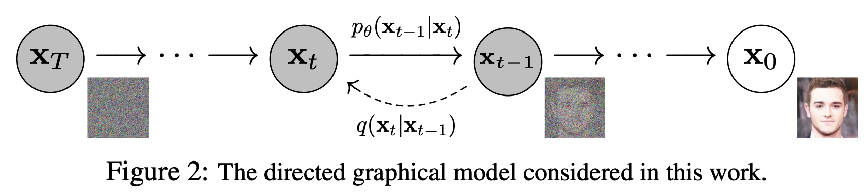 Figure 1: An Overview of the DDPM Framework
Forward Process
The forward process of DDPM begins by sampling a data point \( x_0 \sim q_{\text{data}} \) from the true data distribution. As the continuous time \( t \) progresses, a faint Gaussian noise is gradually added to the data \( x_0 \), with its standard deviation and variance determined by \( \beta_t \). Specifically, the forward process generates a series of images \( x_1, \ldots, x_T \) with noise continuously injected. When \( T \) approaches infinity, \( x_T \) can be considered as belonging to an independent Gaussian distribution \( \mathcal{N}(0, \mathbf{I}) \). The mathematical definition of the forward process is as follows:
$$ q(x_t | x_{t-1}) = \mathcal{N}(x_t; \sqrt{1 - \beta_t} x_{t-1}, \beta_t I) $$Since the forward process of DDPM is built on a Markov chain, we can define the joint probability distribution of the entire process as:
$$ q(x_{1:T} | x_0) = \prod_{t=1}^{T} q(x_t | x_{t-1}) $$Using the reparameterization trick and the properties of the Markov chain, we can derive:
$$ x_t = \sqrt{\bar{\alpha}_t} x_0 + \sqrt{1 - \bar{\alpha}_t} z $$Furthermore, through reparameterization, we can obtain the marginal probability distribution of the noisy data:
$$ q(x_t | x_0) = \mathcal{N}(x_t; \sqrt{\bar{\alpha}_t} x_0, (1 - \bar{\alpha}_t) I) $$This marginal probability distribution is the key target of the DDPM forward process modeling. That is to say, given any \( x_0 \sim q_{\text{data}} \), we can obtain the noisy data \( x_t \). However, the main goal of DDPM is to learn to generate images. Next, we will introduce how to derive the image generation objective function of the model based on the forward process, that is, the reverse process.
Reverse Process
Before engaging in the reverse process inference, let us first clarify the objective of this process. If we intend to fit the reverse process with a model network, it is imperative to deduce the formula of the reverse process, which must encompass the unknown variables that the model seeks to derive. Why is this the case? If we already knew the specific formula and every variable within \( q(x_{t-1}|x_t) \), there would be no need for fitting.
Upon examining the formula for the reverse process, it is evident that we require the distribution outcomes for \( x_t \) and \( x_{t-1} \). Since \( x_0 \) does not influence \( x_t \) and \( x_{t-1} \), it follows that \( q(x_{t-1}|x_t) = q(x_{t-1}|x_t,x_0) \). By integrating Bayes’ theorem with the marginal probability distribution \( q(x_t|x_0) \), we can establish the following:
$$ \begin{align*} q(x_{t-1}|x_t,x_0) &= q(x_t|x_{t-1},x_0) \frac{q(x_{t-1}|x_0)}{q(x_t|x_0)} \\ & \propto exp(\frac{1}{2}(\frac{x_t-\sqrt{\alpha_t}x_{t-1}}{\beta_t}+\frac{(x_{t-1}-\sqrt{\bar{\alpha}_{t-1}}x_0)^2}{1-\bar{\alpha}_{t-1}}-\frac{(x_t-\sqrt{\bar{\alpha}_t}x_0)^2}{1-\bar{\alpha_t}})) \\ &= exp(-\frac{1}{2} ((\frac{\alpha_t}{\beta_t}+\frac{1}{1-\bar{\alpha}_{t-1}})x_{t-1}^2-(\frac{2\sqrt{\alpha_t}}{\beta_t}+\frac{2\sqrt{\bar{\alpha}_t}}{1-\bar{\alpha}_{t-1}}x_0)x_{t-1}+C(x_t,x_0))) \end{align*} $$Where \( C(x_t, x_0) \) is an expression independent of \( x_{t-1} \), we can deduce the coefficients of the quadratic equation as follows:
$$ \tilde{\beta}_t = \frac{1-\bar{\alpha}_{t-1}}{1-\bar{\alpha}_t} \cdot \beta_t \\ \tilde{\mu}_t (x_t,x_0) = \frac{\sqrt{\alpha_t}(1-\bar{\alpha}_{t-1})}{1-\bar{\alpha}_t}x_{t} + \frac{\sqrt{\bar{\alpha}_{t-1}}\beta_t}{1-\bar{\alpha}_t}x_0 $$In the process of constructing mathematical models, we often face choices: when substituting the variable \( x_0 \), we obtain the mean expression \( \tilde{\mu}_t = \frac{1}{\sqrt{\alpha_t}} \left( x_t - \frac{\beta_t}{\sqrt{1-\bar{\alpha}_t}} z_t \right) \). Which one should we actually use? In fact, we need to consider both. During the training phase, since \( x_0 \) is known, we naturally tend to use the first expression. In the generation phase, \( x_0 \) is unknown, making the second expression particularly important. They are not mutually exclusive but show different applicability depending on the application scenario. The choice depends on whether our dataset is already clear.
Having derived the formula for the reverse diffusion process, we now need to fit the distribution derived from \( q(x_{t-1}|x_t,x_0) \) with the conditional probability \( p_\theta(x_{t-1}|x_t) \). So, how do we fit to construct the loss function? Obviously, this is a likelihood-based model problem. The loss function is derived by constructing a variational lower bound. There are mainly two derivation methods: one is to construct the Kullback-Leibler (KL) divergence based on the logarithmic likelihood \( \log p(x_0) \); the other is to use Jensen’s inequality for derivation. The following will show the derivation process of the second method, namely the calculation formula for \( L_{\text{VLB}} \) as follows:
$$ \begin{align*} L_{CE} &= -\mathbb{E}_{q(x_0)} \log p_\theta(x_0) \\ &= -\mathbb{E}_{q(x_0)} \log \left( \int p_\theta(x_{0:T}) dx_{1:T} \right) \\ &= -\mathbb{E}_{q(x_0)} \log \left( \mathbb{E}_{q(x_{1:T}|x_0)} \frac{p_\theta(x_{0:T})}{q(x_{1:T}|x_0)} \right) \\ & \le -\mathbb{E}_{q(x_{0:T})} \log \frac{p_\theta(x_{0:T})}{q(x_{1:T}|x_0)} \\ &= \mathbb{E}_q(x_{0:T})\left[ \log \frac{q(x_{1:T}|x_0)}{p_\theta(x_{0:T})} \right] = L_{\text{VLB}} \end{align*} $$Expanding \(L_{\text{VLB}}\), the derivation process is illustrated as follows:
$$ \begin{array}{l}L_{\mathrm{VLB}}=\mathbb{E}_{q\left(\mathbf{x}_{0: T}\right)}\left[\log \frac{q\left(\mathbf{x}_{1: T} \mid \mathbf{x}_{0}\right)}{p_{\theta}\left(\mathbf{x}_{0: T}\right)}\right] \\ =\mathbb{E}_{q}\left[\log \frac{\prod_{t=1}^{T} q\left(\mathbf{x}_{t} \mid \mathbf{x}_{t-1}\right)}{p_{\theta}\left(\mathbf{x}_{T}\right) \prod_{t=1}^{T} p_{\theta}\left(\mathbf{x}_{t-1} \mid \mathbf{x}_{t}\right)}\right] \\ =\mathbb{E}_{q}\left[-\log p_{\theta}\left(\mathbf{x}_{T}\right)+\sum_{t=1}^{T} \log \frac{q\left(\mathbf{x}_{t} \mid \mathbf{x}_{t-1}\right)}{p_{\theta}\left(\mathbf{x}_{t-1} \mid \mathbf{x}_{t}\right)}\right] \\ =\mathbb{E}_{q}\left[-\log p_{\theta}\left(\mathbf{x}_{T}\right)+\sum_{t=2}^{T} \log \frac{q\left(\mathbf{x}_{t} \mid \mathbf{x}_{t-1}\right)}{p_{\theta}\left(\mathbf{x}_{t-1} \mid \mathbf{x}_{t}\right)}+\log \frac{q\left(\mathbf{x}_{1} \mid \mathbf{x}_{0}\right)}{p_{\theta}\left(\mathbf{x}_{0} \mid \mathbf{x}_{1}\right)}\right] \\ =\mathbb{E}_{q}\left[-\log p_{\theta}\left(\mathbf{x}_{T}\right)+\sum_{t=2}^{T} \log \left(\frac{q\left(\mathbf{x}_{t-1} \mid \mathbf{x}_{t}, \mathbf{x}_{0}\right)}{p_{\theta}\left(\mathbf{x}_{t-1} \mid \mathbf{x}_{t}\right)} \cdot \frac{q\left(\mathbf{x}_{t} \mid \mathbf{x}_{0}\right)}{q\left(\mathbf{x}_{t-1} \mid \mathbf{x}_{0}\right)}\right)+\log \frac{q\left(\mathbf{x}_{1} \mid \mathbf{x}_{0}\right)}{p_{\theta}\left(\mathbf{x}_{0} \mid \mathbf{x}_{1}\right)}\right] \\ =\mathbb{E}_{q}\left[-\log p_{\theta}\left(\mathbf{x}_{T}\right)+\sum_{t=2}^{T} \log \frac{q\left(\mathbf{x}_{t-1} \mid \mathbf{x}_{t}, \mathbf{x}_{0}\right)}{p_{\theta}\left(\mathbf{x}_{t-1} \mid \mathbf{x}_{t}\right)}+\sum_{t=2}^{T} \log \frac{q\left(\mathbf{x}_{t} \mid \mathbf{x}_{0}\right)}{q\left(\mathbf{x}_{t-1} \mid \mathbf{x}_{0}\right)}+\log \frac{q\left(\mathbf{x}_{1} \mid \mathbf{x}_{0}\right)}{p_{\theta}\left(\mathbf{x}_{0} \mid \mathbf{x}_{1}\right)}\right] \\ =\mathbb{E}_{q}\left[-\log p_{\theta}\left(\mathbf{x}_{T}\right)+\sum_{t=2}^{T} \log \frac{q\left(\mathbf{x}_{t-1} \mid \mathbf{x}_{t}, \mathbf{x}_{0}\right)}{p_{\theta}\left(\mathbf{x}_{t-1} \mid \mathbf{x}_{t}\right)}+\log \frac{q\left(\mathbf{x}_{T} \mid \mathbf{x}_{0}\right)}{q\left(\mathbf{x}_{1} \mid \mathbf{x}_{0}\right)}+\log \frac{q\left(\mathbf{x}_{1} \mid \mathbf{x}_{0}\right)}{p_{\theta}\left(\mathbf{x}_{0} \mid \mathbf{x}_{1}\right)}\right] \\ =\mathbb{E}_{q}\left[\log \frac{q\left(\mathbf{x}_{T} \mid \mathbf{x}_{0}\right)}{p_{\theta}\left(\mathbf{x}_{T}\right)}+\sum_{t=2}^{T} \log \frac{q\left(\mathbf{x}_{t-1} \mid \mathbf{x}_{t}, \mathbf{x}_{0}\right)}{p_{\theta}\left(\mathbf{x}_{t-1} \mid \mathbf{x}_{t}\right)}-\log p_{\theta}\left(\mathbf{x}_{0} \mid \mathbf{x}_{1}\right)\right] \\ =\mathbb{E}_{q}[\underbrace{D_{\mathrm{KL}}\left(q\left(\mathbf{x}_{T} \mid \mathbf{x}_{0}\right) \| p_{\theta}\left(\mathbf{x}_{T}\right)\right)}_{L_{T}}+\sum_{t=2}^{T} \underbrace{D_{\mathrm{KL}}\left(q\left(\mathbf{x}_{t-1} \mid \mathbf{x}_{t}, \mathbf{x}_{0}\right) \| p_{\theta}\left(\mathbf{x}_{t-1} \mid \mathbf{x}_{t}\right)\right)-\log p_{\theta}\left(\mathbf{x}_{0} \mid \mathbf{x}_{1}\right)}_{L_{t-1}}] \\\end{array} $$When delving deeper into the construction of the loss function for the reverse diffusion process, we note that \( L_{t-1} \) is a key component of \( L_{\text{VLB}} \), which relies on the dynamic changes of variables, while \( L_{T} \), as a constant term, can be disregarded in calculations. Next, let’s expand \( L_{t} \), the transition from \( t-1 \) to \( t \), with the following expression:
$$ L_{t-1} = \mathbb{E}_q\left[\frac{1}{2\sigma_t^2} \left\| \tilde{\mu}_t(x_t,x_0) - \mu_\theta(x_t,t) \right\|^2 \right] + C $$This formula is primarily constructed based on the objective of mean modeling. However, in addition to the mean, we can also target the noise or the original image itself for modeling. By further substituting \( \mu \) and simplifying, we obtain a simplified loss function:
$$ \begin{align*} L_{\text{simple}}(\theta) &= \mathbb{E}_q\left[\left\| \epsilon - \epsilon_\theta(x_t,t) \right\|^2 \right] \\ &= \mathbb{E}_q\left[\left\| \epsilon - \epsilon_\theta\left(\sqrt{\bar{\alpha}_t}x_0 + \sqrt{1-\bar{\alpha}_t}\epsilon, t\right) \right\|^2 \right] \end{align*} $$The above introduces the mathematical reasoning part of DDPM. Although the mathematical reasoning process of DDPM may seem complex, we ultimately arrive at a concise and clear loss function, which provides a solid foundation for training diffusion models.
Training and Sample Process
The objective function of DDPM is a simple Gaussian noise mean square error prediction. However, due to the concept of time step \( t \) in the mathematical definition of DDPM, its training process needs to consider the prediction of Gaussian noise at each time step, and the same applies to the sampling process. The specific details are shown in the figure below.
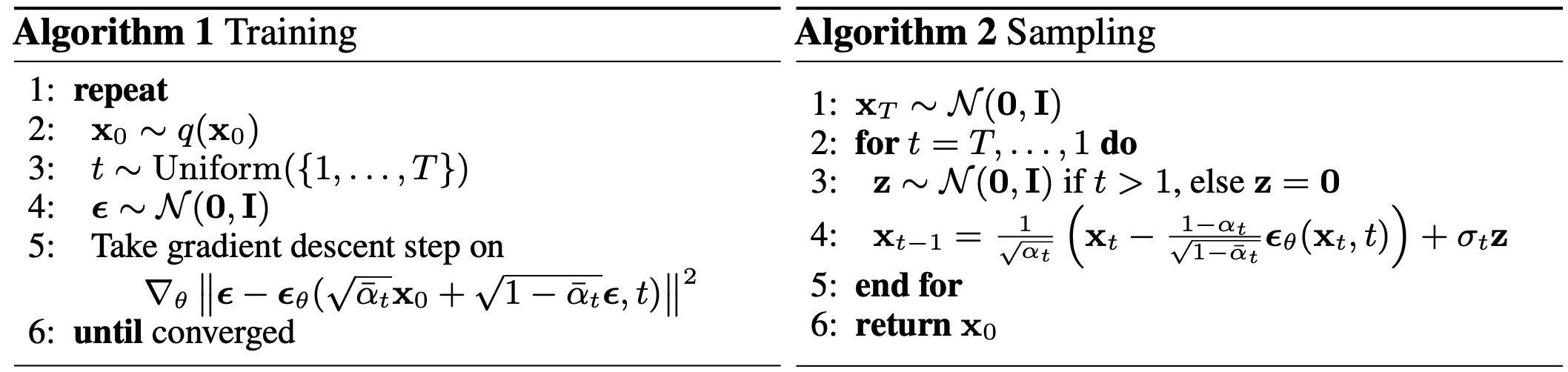 Figure 2: The training and sampling algorithm of DDPM
DDIM
Accelerate Generation Process
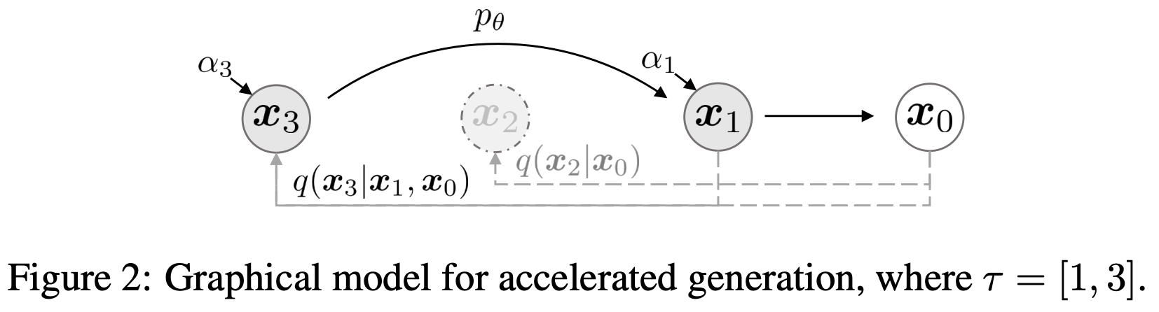
The reverse diffusion process of DDIM significantly differs from that of DDPM. Unlike the step-by-step retrogression of DDPM from step \( t \) to \( t-1 \), DDIM first reverts from step \( t \) back to the initial state \( x_0 \), and then predicts \( x_{t-1} \) based on \( x_t \) and \( x_0 \). It’s worth noting that although DDPM could theoretically perform an operation that jumps to \( x_0 \), the original paper did not adopt this method. In DDIM, the predicted \( x_0 \) is referred to as the denoised observation, and its mathematical expression is defined as follows:
$$ f_\theta^{(t)}(x_t) := \frac{x_t - \sqrt{1 - \alpha_t} \cdot \epsilon_\theta^{(t)}}{\sqrt{\alpha_t}} $$Given a fixed prior \( p_\theta(x_T) = \mathcal{N}(0, I) \), we can determine the objective for the neural network to approximate the reverse diffusion process, with the expression given by:
$$ p_\theta^{(t)}(x_{t-1} | x_t) = \begin{cases} \mathcal{N}(f_\theta^{(1)}(x_1), \sigma_1^2 I), & \text{if } t = 1 \\ q_\sigma(x_{t-1} | x_t, f_\theta^{(t)}(x_t)), & \text{otherwise} \end{cases} $$After establishing the target for the neural network approximation, we further explore the results of the sampled \( x_{t-1} \). Reviewing the diffusion process’s \( q(x_{t-1} | x_0) \), we have proven that this distribution follows a normal distribution, thus allowing the use of the reparameterization trick for expression:
$$ x_{t-1} = \sqrt{\alpha_{t-1}} x_0 + \sqrt{1 - \alpha_{t-1}} \epsilon_\theta^{(t)}(x_t) $$According to the properties of the Gaussian distribution, i.e., \( x + y \sim \mathcal{N}(0, \sqrt{a^2 + b^2}) \), we can split the second term in the above equation:
$$ x_{t-1} = \sqrt{\alpha_{t-1}} x_0 + \sqrt{1 - \alpha_{t-1} - \sigma_t^2} \epsilon_\theta^{(t)}(x_t) + \sigma_t \epsilon_t $$Here, \( \epsilon_\theta^{(t)}(x_t) \) and \( \epsilon_t \) are both random variables from a Gaussian distribution. Further substituting the expression for \( x_0 \) :
$$ x_0 = \frac{1}{\sqrt{\alpha_t}} \left( x_t - \sqrt{1 - \alpha_t} \epsilon_\theta^{(t)}(x_t) \right) $$After substituting \( x_0 \), we obtain:
$$ x_{t-1} = \sqrt{\alpha_{t-1}} \frac{1}{\sqrt{\alpha_t}} \left( x_t - \sqrt{1 - \alpha_t} \epsilon_\theta^{(t)}(x_t) \right) + \sqrt{1 - \alpha_{t-1} - \sigma_t^2} \epsilon_\theta^{(t)}(x_t) + \sigma_t \epsilon_t $$Specifically, in DDPM, \( x_{t-1} \) is obtained through the reparameterization of \( p_\theta(x_{t-1} | x_t) \), while in DDIM, \( x_{t-1} \) is derived based on the diffusion process. This actually verifies the correctness of the author’s proposed \( q_\sigma(x_{t-1} | x_t, x_0) \).
Sample Process without Intermediate Noise
Although DDIM is not based on a Markov chain, its training process is consistent with that of DDPM. That is, the DDPM model can be used for accelerated inference without retraining, reducing from 1000 steps to 50. Specifically, the sampling formula for DDIM can be defined as:
$$ q_{\sigma}\left(\boldsymbol{x}_{\tau_{i-1}} \mid \boldsymbol{x}_{\tau_i}, \boldsymbol{x}_{0}\right)=\mathcal{N}\left(\sqrt{\alpha_{\tau_{i-1}}} \boldsymbol{x}_{0}+\sqrt{1-\alpha_{\tau_{i-1}}-\sigma_{\tau_i}^{2}} \cdot \frac{\boldsymbol{x}_{\tau_i}-\sqrt{\alpha_{\tau_i}} \boldsymbol{x}_{0}}{\sqrt{1-\alpha_{\tau_i}}}, \sigma_{\tau_i}^{2} \boldsymbol{I}\right) $$In the sampling process of DDIM, it is common to set \( \sigma = 0 \). As shown in the figure, the sampling time steps of DDIM are not continuous; it uses \( x_0 \) as a stepping stone and can jump from \( x_3 \) to \( x_1 \).
Reference
[1]Ho, J., Jain, A., & Abbeel, P. (2020). Denoising diffusion probabilistic models. Advances in neural information processing systems, 33, 6840-6851.
[2]Song, J., Meng, C., & Ermon, S. (2020). Denoising diffusion implicit models. arXiv preprint arXiv:2010.02502.