Score-based Generative Model

The content introduced in this article pertains to SMLD, NCSN, DDPM, and SDEs. Before we proceed with the main body of the article, I will first clarify the specific relationships among these concepts for the readers. The SMLD model, proposed by Dr. Song in his 2019 thesis, is a generative method primarily composed of score matching and Langevin dynamics sampling. Given that this method has certain limitations—details of which are presented in the mathematical reasoning section—the author introduced the NCSN method as an improvement. DDPM, the Denoising Diffusion Probabilistic Model, was introduced by Ho et al. in 2020, and it is distinguished from SMLD by its noise addition approach. SDEs refer to the Stochastic Differential Equations used by Dr. Song in his 2021 paper to theoretically evolve the discrete noise addition processes of SMLD and DDPM into a continuous form, thereby unifying the sampling equations of SMLD and DDPM with SDEs. With this brief introduction complete, let us now move on to the section on mathematical reasoning.

Score-Based Generative Modeling

Score Function

The objective of generative tasks is to fit the model parameters to approximate the true data probability distribution \( p(x) \). This probability distribution is typically modeled as \( p_\theta(x) = \frac{e^{-f_\theta(x)}}{Z_\theta} \), where \( f_\theta(x) \in \mathbb{R} \) and \( Z_\theta \) is the normalization term that ensures \( p_\theta(x) \) falls within the probability range. The above distribution is generally referred to as an unnormalized probabilistic model. Our goal is to maximize \( \log p_\theta(x) \) through the log-likelihood method. However, since \( Z_\theta \) is an unknown quantity, we cannot derive \( \log p_\theta(x) \), and thus we cannot optimize the model parameters.

To address the issue of the incalculable \( Z_\theta \), the authors propose the score function, which is defined by the following formula:

$$ s_\theta(x) = \nabla_x \log p_\theta(x) = - \nabla_x f_\theta(x) - \nabla_x \log Z_\theta = -\nabla_x f_\theta(x) $$

We can observe that the score function \( s_\theta(x) \) is independent of \( Z_\theta \), thus circumventing the problem of the unknown \( Z_\theta \). With the known \( s_\theta(x) \), we can construct a loss function to approximate \( s(x) \), thereby accomplishing the generative task.

Score Matching

Score matching, which includes denoising score matching and sliced score matching, is a technique used in generative modeling. Since we will be consistently referring to denoising score matching in the following context, we will use this term. With this, we have our loss function defined as:

$$ \mathcal{L} = \mathbb{E}_{p(x)} \left[ \left\| \nabla_x \log p(x) - s_\theta(x) \right\|^2 \right] $$

If we knew the true distribution \( p(x) \), we could optimize this loss function. However, since we do not, the authors introduced score matching, a method that minimizes the loss function without knowing \( p(x) \), making \( \mathcal{L} \) equivalent to another form:

$$ \mathcal{L} = \mathbb{E}_{p(x)} \left[ \left\| s_\theta(x) \right\|^2 + 2 \text{tr}(\nabla_x s_\theta(x)) \right] $$

To briefly explain the derivation, we expand the expectation, break down the quadratic form, and obtain:

$$ \mathcal{L} = \int p(x) \left[ \left\| \nabla_x \log p(x) \right\|^2 + \left\| s_\theta(x) \right\|^2 - 2(\nabla_x \log p(x))^T s_\theta(x) \right] dx $$

This expression contains three terms. The first term does not involve \( \theta \) and can be ignored. The second term is \( \int p(x) \left\| s_\theta(x) \right\|^2 dx \), and the third term, after manipulation, becomes \( 2 \int p(x) \text{tr}(\nabla_x s_\theta(x)) dx \) after integration by parts.

Looking back at the loss function, \( \nabla_x s_\theta(x) \) represents the Jacobian matrix of \( s_\theta(x) \), which is computationally complex. Can we avoid computing the Jacobian matrix? The authors cleverly used denoising score matching, which perturbs the data \( x \) with a fixed noise distribution to obtain \( q_\sigma(\tilde{x}|x) \). The loss function then becomes:

$$ \mathcal{L} = \mathbb{E}_{p(x)} \left[ \left\| \nabla_{\tilde{x}} \log q_\sigma(\tilde{x}|x) - s_\theta(\tilde{x}) \right\|^2 \right] $$

Now, since \( q_\sigma(\tilde{x}|x) \) is known, we can directly optimize to obtain \( s_{\theta^*}(x) = \nabla_x \log q_\sigma(x) \); clearly, when the added noise is sufficiently small, we can assume \( s_{\theta^*}(x) = \nabla_x \log q_\sigma(x) \approx \nabla_x \log p_{\text{data}}(x) \).

With this, we have completed the optimization of the score-based model, which can help us accomplish a series of generative tasks. So, how should we use it to enable random noise to be restored to an image close to the true data distribution?

Langevin Dynamics Sample

To recover an image close to the true data distribution from random noise, one can employ Langevin dynamics sampling. This sampling method can transform random noise, which follows any distribution, into an image. Langevin dynamics sampling can perform sampling from a probability density function \( p(x) \) based solely on the score function \( \nabla_x \log p(x) \). Given a fixed step size \( \epsilon > 0 \) and an initial noise \( \tilde{x} \sim \pi(x) \), where \( \pi \) can be any distribution, the formula for Langevin dynamics sampling is as follows:

$$ \tilde{x}_t = \tilde{x}_{t-1} + \frac{\epsilon}{2} \nabla_x \log p(\tilde{x}_{t-1}) + \sqrt{\epsilon} z_t $$

Here, \( z_t \sim \mathcal{N}(0, I) \). As \( \epsilon \rightarrow 0 \) and \( T \rightarrow \infty \), the distribution of \( \tilde{x}_T \) equals \( p(x) \). It is not difficult to see that the above formula only requires \( \nabla_x \log p(x) \). Therefore, to generate samples close to the distribution \( p_{\text{data}}(x) \), we can first train a score model \( s_\theta(x) \approx \nabla_x \log p_{\text{data}}(x) \) .

With this, we have obtained a model composed of score matching and Langevin dynamics sampling, hence called the SMLD (Score Matching Langevin Dynamics) model. However, this model actually has significant issues. Let’s now examine what these problems are and how the authors addressed them.

Noise Conditional Score Networks

Let’s first examine the loss function of the SMLD model, where the issue arises:

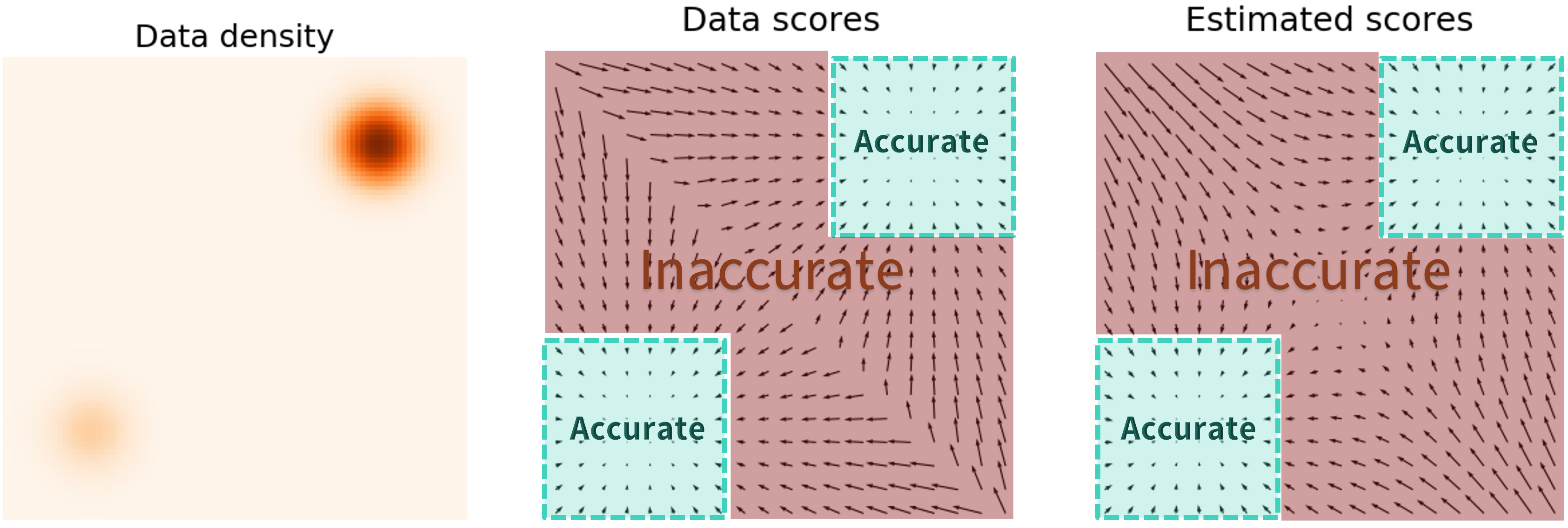
$$ \mathcal{L} = \mathbb{E}_{p(x)} \left[ \left\| \nabla_x \log p(x) - s_\theta(x) \right\|^2 \right] = \int p(x) \left\| \nabla_x \log p(x) - s_\theta(x) \right\|^2 dx $$

It is evident that \( p(x) \) acts as a weight on the L2 term. Consequently, when \( p(x) \) reaches areas of low density, the L2 term loses its effectiveness as a loss function. In these regions, the estimated score model \( s_\theta(x) \) becomes inaccurate, as illustrated in the figure below. The predicted scores closely match the actual data scores in high-density areas, but they are inaccurate in low-density areas. If this issue is not addressed, it becomes impossible to generate samples that conform to the true distribution.

To address this problem, the authors proposed improvements to the score matching approach. One such improvement is to use a different weighting scheme that does not depend on the density of \( p(x) \) in areas where the density is low. This can be achieved by employing alternative loss functions that penalize deviations of the score estimates more uniformly across the sample space, regardless of the local density of \( p(x) \). By doing so, the model can learn to accurately represent the score function even in low-density regions, thus improving the generative capabilities of the model and enabling it to produce samples that better reflect the true data distribution.

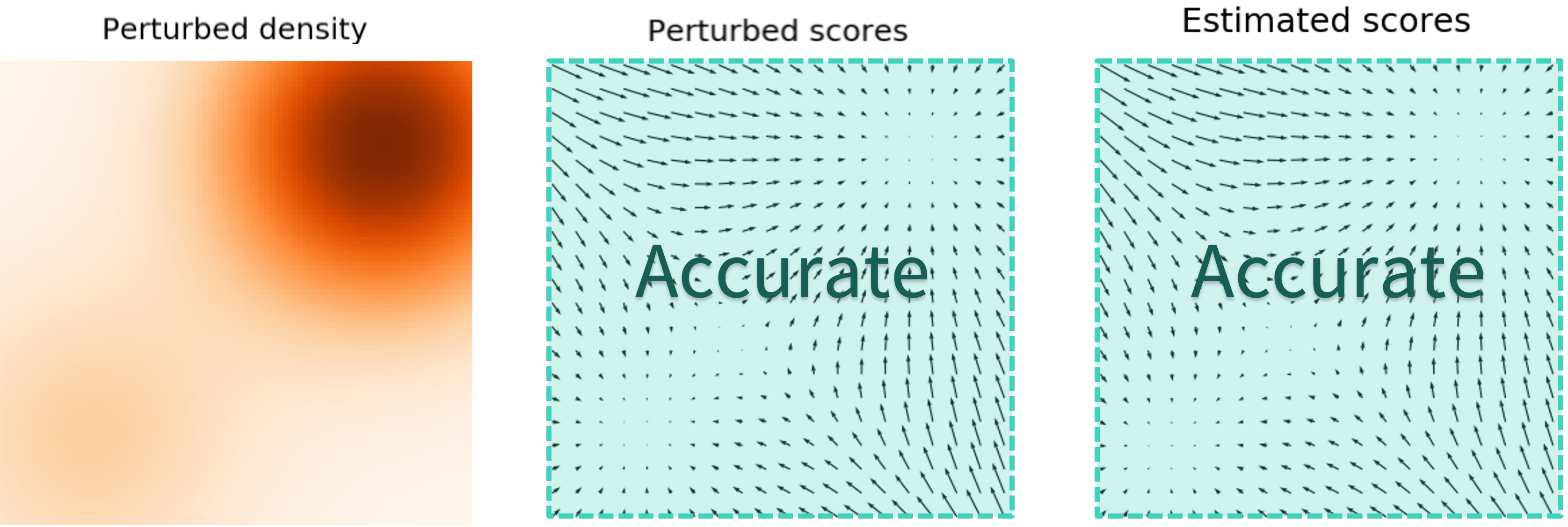
To address the issue, the authors introduced Noise Conditional Score Networks (NCSN), which expands the high-density area of the data distribution by adding noise perturbations to the data. By superimposing Gaussian noise on the data distribution, the mean remains unchanged while the variance increases, effectively enlarging the area of the high-density region. This enlargement allows for more accurate estimation of the score function in a broader range of areas.

Once the approach of adding noise is established, we must consider whether to add noise once or multiple times, and whether to add a small or large amount of noise. Clearly, if the noise perturbation is small, it will not significantly affect the data distribution; conversely, if the noise perturbation is large, it will alter the original data distribution. Therefore, the authors propose a compromise: to add noise multiple times, starting small and increasing in intensity. We define a sequence \(\{ \sigma_i \}_{i=1}^L\), with \(\sigma_1 < \sigma_2 < ... < \sigma_L\), representing noise intensities from low to high. This allows us to define the distribution of the data after noise perturbation as follows:

$$ x + \sigma_i z \sim p_{\sigma_i}(x) = \int p(y) \mathcal{N}(x|y, \sigma_i^2I)dy $$

We then estimate a series of score functions for the noise-perturbed distributions and sum them to obtain:

$$ \mathcal{L} = \sum_{i=1}^L \sigma_i^2 \ \mathbb{E}_{p(x)} \left[ \left\| \nabla_{\tilde{x}} \log p_{\sigma_i}(x) - s_\theta(x) \right\|^2 \right] $$

For the training of NCSN, using denoising score matching, we define the noise distribution as \( q_\sigma(\tilde{x}|x) = \mathcal{N}(\tilde{x}|x,\sigma^2I) \), hence the score function \( \nabla_{\tilde{x}} \log q_{\sigma}(\tilde{x}|x) = -(\tilde{x}-x)/\sigma^2 \). Given a \( \sigma \), the loss function for NCSN can be written as:

$$ l(\theta;\sigma) := \frac{1}{2} \mathbb{E}_{p_{\text{data}}(x)} \mathbb{E}_{\tilde{x} \sim \mathcal{N}(x, \sigma^2I)} \left[ \left\| s_\theta(\tilde{x}, \sigma) + \frac{\tilde{x}-x}{\sigma^2} \right\|^2 \right] $$

With the loss function for a single noise level, we can derive the formula for all noise levels:

$$ \mathcal{L}(\theta;\{\sigma_i \}_{i=1}^L) := \frac{1}{L} \sum_{i=1}^L \lambda(\sigma_i)l(\theta; \sigma_i) $$

Given that \( s_{\theta^*}(x,\sigma_i) = \nabla_x \log q_{\sigma_i}(x) \), the optimization of the loss function is completed. Note that the input to the score model is not only \( x \) but also the noise intensity \( \sigma_i \). It is important to clarify that \( \lambda(\sigma_i) \) is a coefficient function that depends on \( \sigma_i \), and there are various ways to choose it. The authors wish for the different noise loss functions \( \lambda(\sigma) l(\theta; \sigma) \) to be on the same scale. Through “experimental observation,” it was found that \( \lVert s_\theta(x, \sigma) \rVert \propto 1/\sigma \). Therefore, the authors set \( \lambda(\sigma) = \sigma^2 \) to ensure that different \( \lambda(\sigma) l(\theta; \sigma) \) are on the same scale, making the loss function independent of the noise level.

For NCSN sampling, instead of direct Langevin dynamics sampling, annealed Langevin dynamics sampling is used. This method, as shown in the figure, performs Langevin dynamics sampling on data distributions with different noise intensities from large to small, using the sampling result of \( L \) as the initial value for the \( L-1 \) sampling. Finally, when \( \sigma_1 \approx 0 \), \( q_{\sigma_1}(x) \) approaches the true data distribution \( p_{\text{data}}(x) \).

From Algorithm 1, it can be seen that the sampling step size \( \alpha_i \) is proportional to the noise intensity; the larger the noise intensity, the larger the sampling step size. Each sampling can obtain \( \tilde{x}_T \), which will serve as the initial value \( \tilde{x}_0 \) for the \( L-1 \) moment. The logic shown in this algorithm is in the order from 1 to \( L \) (here \( \sigma_1 > \sigma_L \), from Dr. Song’s thesis), while my description is the process from \( L \) to 1 ( \( \sigma_1 < \sigma_L \), from Dr. Song’s blog), it’s just a difference in notation; in reality, both are processes from high noise to low noise, so don’t get confused.

Consider why the above sampling method can solve the initial problem of inaccuracy in low-density areas; we can assume that a good sample is drawn from \( q_{\sigma_L}(x) \), which is likely to come from the high-density area of \( q_{\sigma_L}(x) \). Given the small difference between \( q_{\sigma_L}(x) \) and \( q_{\sigma_{L-1}}(x) \), this sample is also very likely to be in the high-density area of \( q_{\sigma_{L-1}}(x) \). Since the score estimation performs better in high-density areas, this sample can be used as the initial value for \( q_{\sigma_{L-1}}(x) \). At this point, some may ask, aren’t you trying to solve the inaccuracy in low-density areas? Why are you always improving the accuracy in high-density areas? Note that the accuracy in the high-density area of \( q_{\sigma_L}(x) \) implies that some low-density areas of \( q_{\sigma_{L-1}}(x) \) are also accurate, doesn’t it? This method ensures the accuracy of low-density areas while also achieving continuous optimization of score estimation in high-density areas.

With this, the content of Dr. Song’s 2019 paper has been introduced. It is not difficult to see that the difference between SMLD (NCSN) and DDPM lies in the different noise addition methods and sampling methods. SMLD (NCSN) involves adding multiple noises to the original image and then restoring the image based on the annealed Langevin sampling method; DDPM involves iteratively adding multiple noises to the original image and then restoring the image based on the Markov chain property to deduce the sampling formula.

Score-Based Models with SDEs

SDEs

Dr. Yang Song’s 2021 paper is based on Stochastic Differential Equations (SDEs) for image diffusion and sampling, an approach that expresses the finite discrete sampling process as an infinite continuous one. The SDE-based method can be seen as a general sampling approach for diffusion models, unifying SMLD and DDPM.

Before delving into the application of SDEs, let’s review the optimization objectives of SMLD and DDPM. The optimization objective for SMLD is:

$$ \boldsymbol{\theta}^{*} = \underset{\boldsymbol{\theta}}{\arg \min } \sum_{i=1}^{N} \sigma_{i}^{2} \mathbb{E}_{p_{\text {data }}(\mathbf{x})} \mathbb{E}_{p_{\sigma_{i}}(\tilde{\mathbf{x}} \mid \mathbf{x})}\left[\left\|\mathbf{s}_{\boldsymbol{\theta}}\left(\tilde{\mathbf{x}}, \sigma_{i}\right)-\nabla_{\tilde{\mathbf{x}}} \log p_{\sigma_{i}}(\tilde{\mathbf{x}} \mid \mathbf{x})\right\|_{2}^{2}\right] $$

The sampling method is the Langevin dynamics sampling formula:

$$ x_i^m = x_i^{m-1} + \epsilon_i s_{\theta^*}(x_i^{m-1}, \sigma_i) + \sqrt{2 \epsilon_i}z_i^m, \ m =1,2,...,M $$

where \( i \) denotes the corresponding noise level, and \( m \) represents the current moment of sampling the image.

The optimization objective for DDPM can also be written in a similar form to SMLD:

$$ \boldsymbol{\theta}^{*} = \underset{\boldsymbol{\theta}}{\arg \min } \sum_{i=1}^{N} (1-\alpha_i) \mathbb{E}_{p_{\text {data }}(\mathbf{x})} \mathbb{E}_{p_{\alpha_{i}}(\tilde{\mathbf{x}} \mid \mathbf{x})}\left[\left\|\mathbf{s}_{\boldsymbol{\theta}}\left(\tilde{\mathbf{x}}, \sigma_{i}\right)-\nabla_{\tilde{\mathbf{x}}} \log p_{\alpha_{i}}(\tilde{\mathbf{x}} \mid \mathbf{x})\right\|_{2}^{2}\right] $$

The sampling method follows the reverse Markov chain:

$$ x_{i-1} = \frac{1}{\sqrt{1-\beta_i}}(x_i + \beta_i s_{\theta^*}(x_i, i)) + \sqrt{\beta_i}z_i, \ i=N,N-1,...,1 $$

The optimization of these two algorithms can be written in the same form, which gives us reason to believe that there may be a unified expression to represent both SMLD and DDPM. So, what is this specific form of expression? Let’s continue to explore.

From discrete to continuous, the forward SDEs perturb the data. When the noise level tends to infinity, we can consider a continuously increasing noise perturbing the original data distribution. In this case, the noise addition process (diffusion process) is a time-continuous stochastic process. The authors propose a concise way to express such stochastic processes, namely SDEs. Why can SDEs be used to represent this? This is because many stochastic processes (especially diffusion processes) are solutions to SDEs. The general formula for SDEs is as follows:

$$ dx = f(x,t)dt + g(t)d \bf{w} $$

Here, \( f: \mathbb{R}^d \rightarrow \mathbb{R}^d \), called the drift coefficient, \( g(t) \in \mathbb{R} \), called the diffusion coefficient, \( \bf{w} \) represents a standard Brownian motion, and \( d \bf{w} \) can be seen as infinitesimally small Gaussian noise. At this point, \( x(t) \) represents the random variable perturbed by noise at time \( t \), and \( p_t(x) \) represents the marginal probability density function of \( x(t) \). Comparing with the finite noise addition, we can consider \( p_t(x) \) similar to \( p_{\sigma_i}(x) \), so \( p_0(x) \) can be considered the original data distribution. When \( T \rightarrow \infty \), we can consider \( p_T(x) \) close to the prior distribution of random noise \( \pi(x) \), which is equivalent to adding the maximum noise perturbation to the data.

SDEs can be artificially designed, similar to how we add noise in NCSN, with the following SDE design:

$$ dx = e^t d \bf{w} $$

This is equivalent to perturbing the data with a Gaussian noise with a mean of 0 and an exponentially increasing variance. (Here, it is stated that \( d\bf{w} \) is an infinitesimal Gaussian distribution). So far, we have designed a noise addition method similar to NCSN based on SDEs, so we have reason to believe that we can express NCSN and DDPM using SDEs.

Reverse SDEs

The reverse SDEs for sample generation were proposed by B.D. Anderson in 1982, stating that every SDE has a corresponding reverse SDE equation, as follows:

$$ dx = [f(x,t) - g^2(t) \nabla_x \log p_t(x)]dt + g(t)d\bf{w} $$

Here, \(dt\) is a negative infinitesimally small time step, and \(t\) is the process from \(T \rightarrow 0\). To solve the reverse SDE, we need to determine the score function \(\nabla_x \log p_t(x)\).

Similar to the NCSN loss function, we can still implement SDE-based score estimation based on the score model and score matching method, replacing the noise in the discrete process at the \(i\)th time with the noise at time \(t\), with the formula as follows:

$$ \mathcal{L}=\mathbb{E}_{t \in \mathcal{U}(0,T)} \mathbb{E}_{p_t(x)} [\lambda(t) \lVert \nabla_x \log p_t(x) - s_\theta(x,t) \rVert^2_2] $$

Here, to ensure that the loss is of the same order at different \(t\) times, let \(\lambda(t) \propto 1/ \mathbb{E} \lVert \log p(x(t)|x(0)) \rVert^2_2\). After optimizing the score model \(s_\theta(x,t)\), substitute it into the reverse SDE:

$$ dx = [f(x,t) - g^2(t)s_\theta(x,t)]dt + g(t)d\bf{w} $$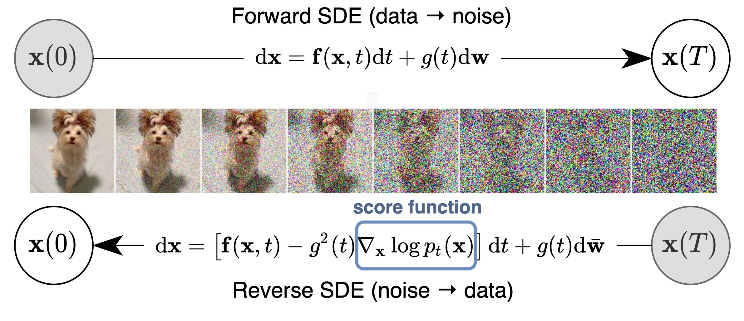

After calculating the specific expression of the reverse SDE, we need to consider how to solve the reverse SDE.

Solving the reverse SDE. We can use numerical methods to solve the reverse SDE, among which the simplest numerical method is the Euler-Maruyama method. This method describes the reverse SDE with finite time steps and infinitesimal Gaussian noise. Specifically, it initializes \(t=T\), \(\nabla_t \approx 0\) (negative time difference), and iterates the following process until \(t \approx 0\):

$$ \begin{align*} \Delta x & \leftarrow [f(x,t) - g^2(t)s_\theta(x,t)] \Delta t + g(t) \sqrt{|\Delta t|}z_t \\ x & \leftarrow x + \Delta x \\ t & \leftarrow t + \Delta t \end{align*} $$

Of course, in addition to this, the author also mentioned other numerical methods, such as the Milstein method and the stochastic Runge-Kutta method. Since the author did not use these methods in the end, they are not elaborated here. Interested friends can study the corresponding papers.

The author proposed a method similar to the Euler-Maruyama method but more suitable for this reverse SDE, which is a method more suitable for this framework, called the predictor-corrector (PC) sampling method.

The PC sampling method can be viewed from two stages. The first stage is prediction, that is, to solve the \(x_i\) of the previous moment by any numerical method. However, due to the existence of errors at this time, the results are inaccurate, so the second stage of correction is needed to adjust the obtained results for \(M\) steps. This stage mainly uses the sampling method in the score model for correction, such as Langevin MCMC. As for the specific sampling formula, we will not discuss it for now, because our goal is not to use a specific SDE to represent SMLD or DDPM. Next, I will introduce how to unify the above two models with SDEs.

SDEs Unify Diffusion Models

For SMLD, by subtracting the noise addition formula at moments \( \sigma_i \) and \( \sigma_{i-1} \), we can obtain the following noise addition method:

$$ x_i = x_{i-1} + \sqrt{\sigma_i^2 - \sigma_{i-1}^2} z_{i-1}, \ z_{i-1} \sim \mathcal{N}(0,I) $$

As the number of noise additions approaches infinity, we can derive:

$$ \begin{align*} x(t + \Delta t) - x(t) &= \sqrt{\frac{d\sigma^2(t)}{dt}} \sqrt{\Delta t} z(t) \\ dx &= \sqrt{\frac{d\sigma^2(t)}{dt}} dw \end{align*} $$

For DDPM, the noise addition method is:

$$ x_i = \sqrt{1-\beta_i}x_{i-1} + \sqrt{\beta_i}z_{i-1}, \ z_{i-1} \sim \mathcal{N}(0, I) $$

As the number of noise additions approaches infinity, we can derive:

$$ dx = -\frac{1}{2} \beta(t)xdt + \sqrt{\beta(t)}dw $$

Since in the noise addition process, the noise in SMLD tends to infinity as \( t \rightarrow \infty \), its corresponding SDE is referred to as a Variance Exploding (VE) SDE. Conversely, the noise in DDPM tends to a boundary value as \( t \rightarrow \infty \), so its corresponding SDE is referred to as a Variance Preserving (VP) SDE.

After determining the SDE representations for SMLD and DDPM, let’s revisit the specific expressions of the PC sampling in the two algorithms, as shown in Algorithm 2, 3.

The prediction phase can use any numerical method to solve the reverse SDE, while the correction phase uses the MCMC method based on the score model. In PC sampling, the predictor and corrector are used alternately. Specifically, the numerical method is used as the predictor, and the annealed Langevin dynamics sampling is used as the corrector.

From SDEs to ODEs. For an SDE, we can express the SDE in an equivalent form based on the Fokker-Planck equation:

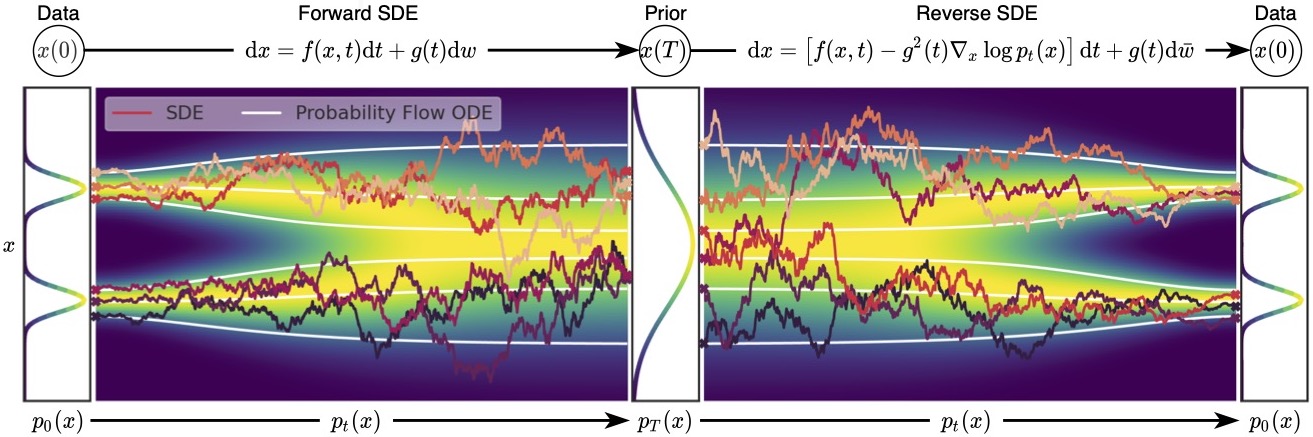
$$ dx = [f(x,t)-\frac{1}{2}(g^2(t)-\sigma^2(t))\nabla_x \log p_t(x)]dt + \sigma(t)d\bf{w} $$

The two SDE formulations are equivalent, hence they share the same marginal probability distribution \( p_t(x) \). If we set \( \sigma(t) = 0 \) in the SDE, we obtain an ordinary differential equation (ODE), commonly referred to as the Probability Flow ODE:

$$ dx = [f(x,t)-\frac{1}{2} g^2(t)\nabla_x \log p_t(x)]dt $$

The figure below illustrates the noise addition and sampling processes of SDEs and Probability Flow ODEs. It can be seen that the trajectory of the Probability Flow ODE is smooth, while the trajectory of the SDE is stochastic, but they share the same marginal distribution. Some may wonder why the Probability Flow ODE is mentioned suddenly, of course, it is because it has advantages over SDEs. For example, ODEs are easier to solve than SDEs, thus faster in sampling; ODEs discard random noise throughout the process, making the process deterministic, allowing for the calculation of probability density. However, ODEs also have disadvantages, such as not generating as well as SDEs.

Additionally, when \( \nabla_x \log p_t(x) \) is replaced by the approximated \( s_\theta(x,t) \), the Probability Flow ODE becomes a special case of a Neural ODE. At the same time, the Probability Flow ODE is also an example of a continuous Flow model because the Probability Flow ODE transforms the data distribution into the prior noise distribution, and the process is reversible. Therefore, the Probability Flow ODE inherits the characteristics of Neural ODEs or continuous Flow models, such as accurate likelihood calculation. We can use numerical ODEs to calculate unknown data distributions from the prior distribution.

Reference

[1] Yang Song, https://yang-song.net/blog/2021/score/.

[2] Song, Y., & Ermon, S. (2019). Generative modeling by estimating gradients of the data distribution. Advances in neural information processing systems, 32.

[3] Song, Y., Sohl-Dickstein, J., Kingma, D. P., Kumar, A., Ermon, S., & Poole, B. (2020). Score-based generative modeling through stochastic differential equations. arXiv preprint arXiv:2011.13456.