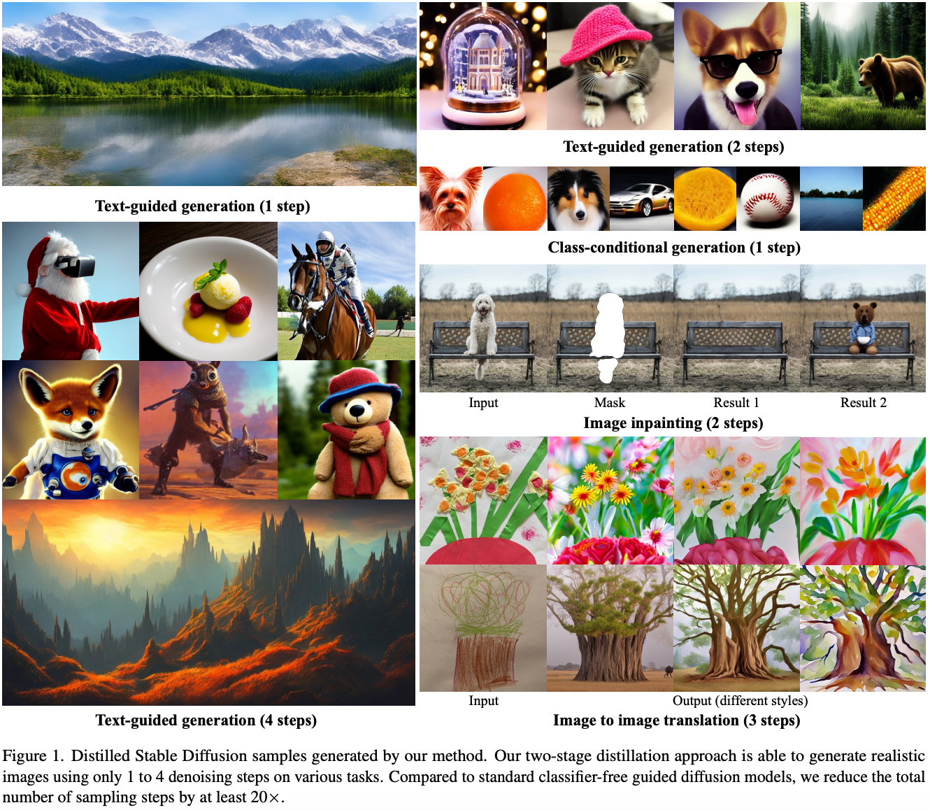
The one-step noise reduction sampling of a student diffusion model that approximates the two- or four-step noise reduction sampling of a teacher model is referred to as progressive distillation. The sampling steps of the student model decrease in the sequence from 128 to 32, then to 8, 4, 2, and finally to 1. Jo, in 2022, introduced Progressive Distillation (PD), marking the inaugural work to propose the ideology of progressive distillation. Subsequently, in 2023, Ho presented On Distillation of Guidance (PGD), which expanded upon the PD methodology on Stable Diffusion and incorporated the concept of distilling the Guidance Scale into the student model. Following this, in 2024, Shi introduced SDXL-Lightning, which integrates adversarial discriminators to boost the performance of the distillation outcomes. In this paper, we will delve into the core principles and training specifics of PD, PGD, and SDXL-Lightning, culminating in a comprehensive summary of the progressive distillation series of research works.
Progressive Distillation
What is progressive distillation?
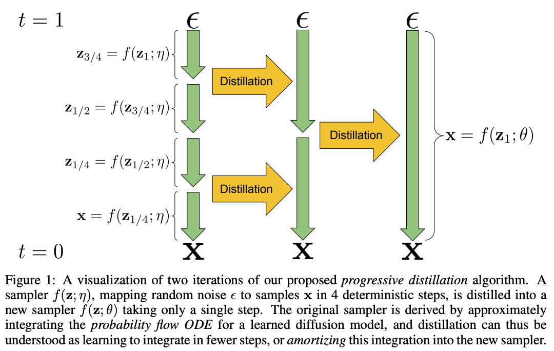
The core idea of progressive distillation is to align the one-step noise reduction sampling of the student model with the two- or four-step noise reduction sampling of the teacher model, significantly reducing the number of sampling steps required by the student model. For instance, given a teacher model \( \epsilon_{\text{tea}}(\cdot) \) and a student model \( \epsilon_{\text{stu}}(\cdot) = \epsilon_{\text{tea}}(\cdot) \), the noisy image obtained after one sampling step by \( \epsilon_{\text{stu}}(\cdot) \), denoted as \( x_{t_{\text{stu}}} \), should approximate the noisy image obtained after two sampling steps by \( \epsilon_{\text{tea}}(\cdot) \), denoted as \( x_{t_{\text{tea}}} \), with \( t_{\text{stu}} = t_{\text{tea}} \). The process of PD is illustrated in the figure below.
Align timesteps of teacher and student model.
To ensure that the student model achieves a sampling result similar to that of the teacher model, it is essential to align the sampling timesteps of \( \epsilon_{\text{tea}}(\cdot) \) and \( \epsilon_{\text{stu}}(\cdot) \). For example, if the teacher model \( \epsilon_{\text{tea}}(\cdot) \) has 32 sampling steps with timesteps set as \( t_{\text{tea}} = [999, 949, 899, ...., 199, 149, 99, 49] \), the student model \( \epsilon_{\text{stu}}(\cdot) \) would have half the number of sampling steps, 16, with timesteps as a subset of \( t_{\text{tea}} \), set as \( t_{\text{stu}} = [999, 899, ..., 199, 99] \) .
Training Process
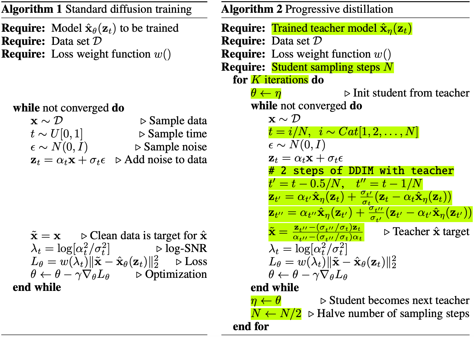
Compared to other recent optimization methods such as consistency distillation, variational score distillation, adversarial training, and reinforcement learning, the training process of PD is straightforward and effective. We will now delve into the details of the PD training process. As shown in Algorithm 1, we obtain true images \( x \) from a dataset of image-text pairs and perform forward diffusion to get \( x_t = \alpha_t x + \sigma_t \epsilon \), where \( \alpha_t \) is the mean, \( \sigma_t \) is the variance, and \( \epsilon \sim \mathcal{N}(0,1) \) .
PD infers and trains from two branches of both a student model and a teacher model. The student model first inputs \( x_t \) into \( \epsilon_{\text{stu}}(\cdot) \) and obtains \( x_{t_{\text{stu-prev1}}} = f_{\text{stu}}(x_t, t_{\text{stu}}, \epsilon_{\text{stu}}, 1) \) through DDIM sampling at one continuous timestep \( t_{\text{stu}} \). Then, in an environment without gradients, the teacher model inputs \( x_t \) into \( \epsilon_{\text{tea}}(\cdot) \) and obtains \( x_{t_{\text{tea-prev2}}} = f_{\text{tea}}(x_t, t_{\text{tea}}, \epsilon_{\text{tea}}, 2) \) through DDIM sampling at two continuous timesteps \( t_{\text{tea}} \). The training objective of PD is to make \( x_{t_{\text{stu-prev1}}} = x_{t_{\text{tea-prev2}}} \), and the training loss can be formulated as:
$$ \mathcal{L}_{PD} = \left[ \left\| x_{t_{\text{stu-prev1}}} - x_{t_{\text{tea-prev2}}} \right\|^2 \right] $$By using a simple MSE loss function, PD achieves the distillation of the quality of the multi-step generated images from the teacher model into the few-step image generation of the student model. The specific training process is shown in the figure below.
Performance about PD.
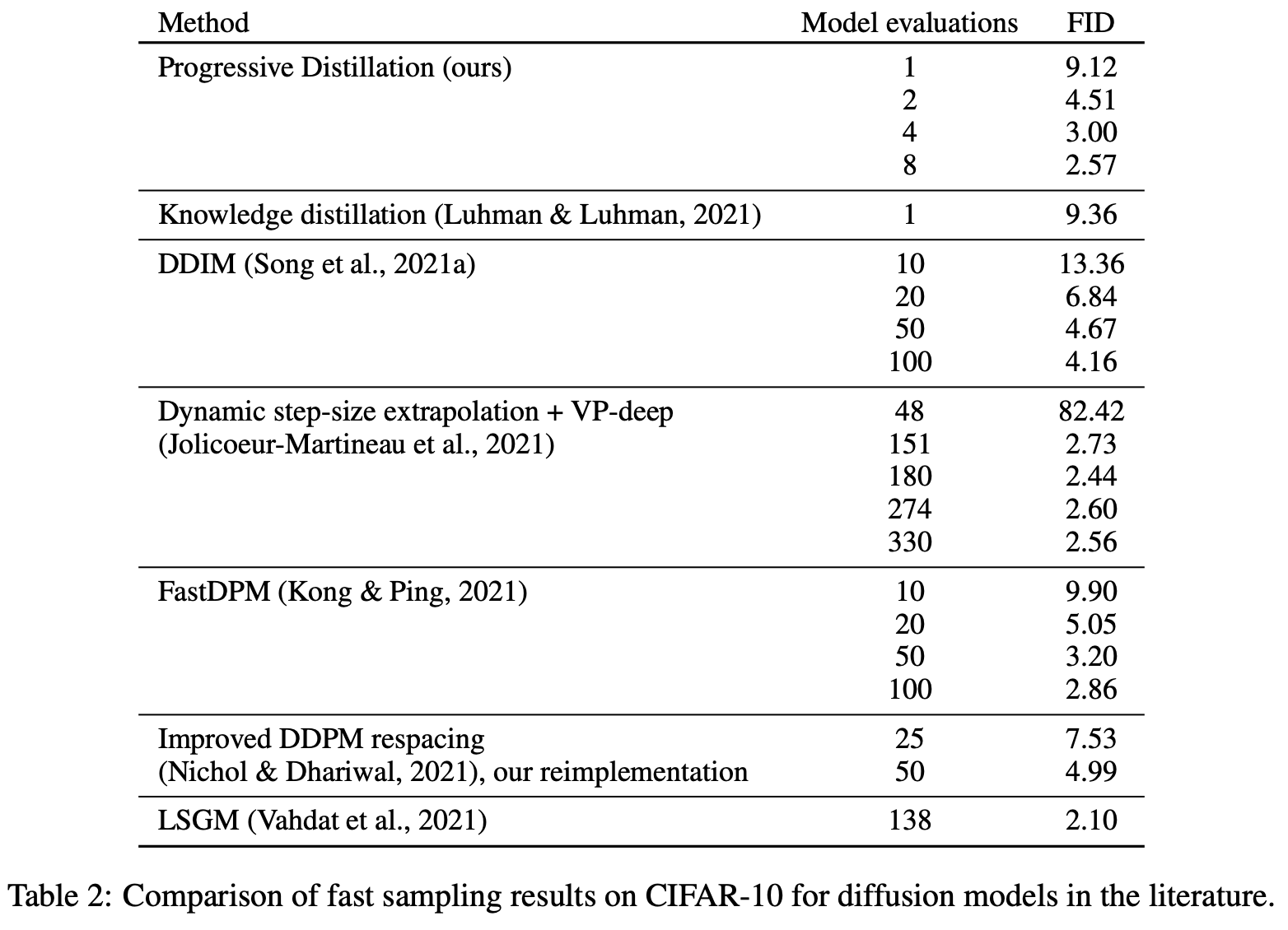
The quantitative performance of PD on CIFAR-10 is shown in the table below. Compared to DDIM, the FID of PD with 2 steps is close to the FID of DDIM with 50 steps of sampling. The performance of PD with 8 steps of sampling is better than that of DDIM with 50 steps. However, in any case, the theoretical upper limit of the student model is the teacher model.
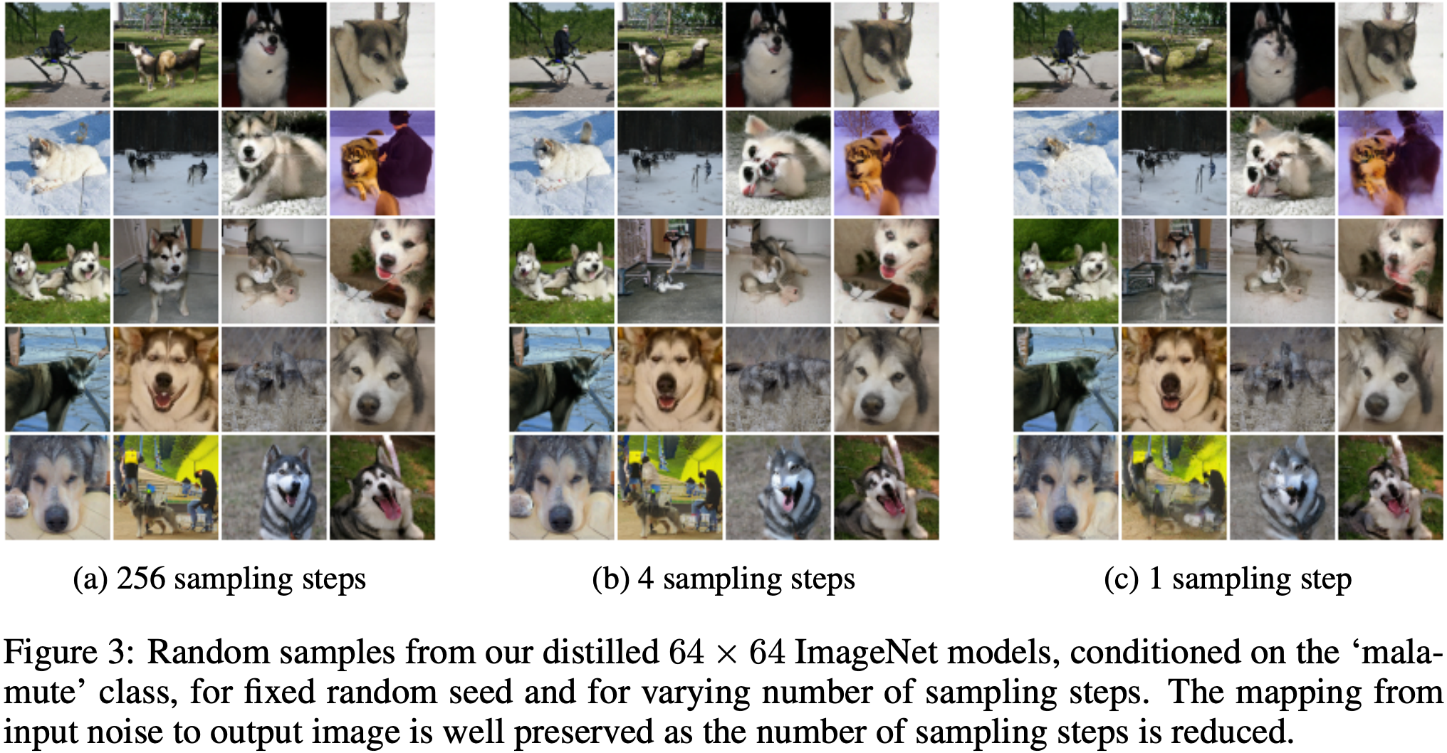
The qualitative experimental results of PD are shown in the figure below. Although PD demonstrates one-step generation performance, there is still a significant gap compared to the 256-step generation performance. In fact, to date, although many one-step inference T2I works have emerged, the number of models that can be implemented is still zero. There is still a great deal of room for optimization in one-step inference of diffusion models.
Progressive Guided Distillation
Training Process
Progressive Guided Distillation (PGD) builds upon the foundation of PD by introducing the Guidance scale \( \omega \) to the distillation of diffusion models. Here, \( \omega \) represents the text guidance strength coefficient proposed in Classifier-free guidance work. Specifically, in the PGD training process, \( w \) is set within the range \( [w_{\text{min}}, w_{\text{max}}] \). The teacher model predicts the noise \( \epsilon_t = \epsilon_{\text{uncond}} + w (\epsilon_{\text{cond}} - \epsilon_{\text{uncond}}) \) at each denoising step and obtains \( x_{t-N} \) after \( N \) steps of inference. For the student model, it directly predicts the conditional noise \( \epsilon_{\text{cond}} \) and obtains \( x_{t-\frac{N}{2} \times 2} \) after \( N/2 \) steps of inference. In this way, the capability of \( \omega \) from the teacher model can be directly distilled into the student model, enabling the student model to achieve similar performance to the teacher model at \( \omega > 1 \) when \( \omega = 1 \).
More generally, in the first phase of distillation, PGD sets \( \omega_{\text{min}} = 5 \) and \( \omega_{\text{max}} = 15 \), obtaining a student model with steps ranging from 128 to 32. Since the capability of \( \omega \) has been distilled into the student model, in the second phase of distillation, PGD sets \( \omega_{\text{min}} = \omega_{\text{max}} = 1 \). The progressive distillation trajectory of PGD is from 32 to 8, 8 to 4, 4 to 2, and finally 2 to 1, resulting in a one-step student model. However, in practical applications, the one-step performance of the student model still does not meet the applicable standards.
SDXL-Lightning
What is SDXL-Lightning?
Progressive distillation is the core method of SDXL-Lightning for accelerating the speed of diffusion sampling. Compared to the works of PD and PGD, the core contribution of SDXL-Lightning is the introduction of a discriminator for adversarial training in progressive distillation, hence the term Progressive Adversarial Distillation. The benchmark model for SDXL-Lightning is SDXL, which is mainly compared with SDXL-Turbo. It is worth mentioning that SDXL-Lightning can still be trained on images of size $1024 \times 1024$ after introducing adversarial training. In contrast, due to memory limitations, SDXL-Turbo can only be trained on images of size $512 \times 512$. The main contribution of SDXL-Lightning is maintaining low memory usage while introducing a discriminator and its optimizer.
Introduce UNet Discriminator to PD.
In adversarial training, the discriminator typically discerns between $x$ and the generated image $x_0$ in the pixel space. Therefore, it is necessary to decode the latent space features to pixel space features $x_0 = D(z_0)$ during training and then input them into the discriminator $d_{\theta}$ for discernment. This process increases the training memory, preventing SDXL-Turbo from training on images of size $1024 \times 1024$.
SDXL-Lightning proposes the use of the UNet Encoder $E$ of the diffusion model as the discriminator, which can directly accept the latent space features $x_t$ and the corresponding timestep $t$ during training. This method eliminates the need for adversarial training in pixel space, effectively reducing training memory and enabling training on images of size $1024 \times 1024$. Specifically, SDXL-Lightning introduces a simple discriminative head on $E$, composed of convolutional and fully connected networks, which outputs a concrete value. The adversarial loss function of SDXL-Lightning, like GAN, consists of the discriminator loss function $L_d$ and the generator loss function $L_g$. After introducing the principles and features of SDXL-Lightning, we will delve into the training process and details of SDXL-Lightning.
Training Process
The training process of SDXL-Lightning primarily differs from that of PD in the loss function used. While PD directly employs an MSE loss function, the loss function of SDXL-Lightning is a combination of the discriminator loss function $L_d$ and the generator loss function $L_g$. Throughout the entire training process, the real and generated inputs of SDXL-Lightning are consistent with those of PD.
The training trajectory of SDXL-Lightning is from 128 to 32, then to 8, 4, 2, and finally to 1. The step from 128 to 32 does not introduce adversarial distillation with the discriminator, while the other processes do include it. During distillation, the Guidance scale is trained into SDXL-Lightning. Therefore, the Guidance scale is set to 1 during inference for SDXL-Lightning. It should be noted that SDXL-Lightning performs distillation at specific timesteps $t$, so the inference timestep strategy must be consistent with the training timestep strategy. For example, the timesteps for a four-step inference should be $[999, 749, 499, 249]$.
Introducing a discriminator for adversarial training is unstable, and it is necessary to incorporate an EMA (Exponential Moving Average) strategy during the training process. Although the EMA strategy is a simple approach, it is very effective in adversarial training.
Reference
[1] Salimans, T., & Ho, J. (2022). Progressive distillation for fast sampling of diffusion models. arXiv preprint arXiv:2202.00512.
[2] Meng, C., Rombach, R., Gao, R., Kingma, D., Ermon, S., Ho, J., & Salimans, T. (2023). On distillation of guided diffusion models. In Proceedings of the IEEE/CVF Conference on Computer Vision and Pattern Recognition (pp. 14297-14306).
[3] Lin, S., Wang, A., & Yang, X. (2024). Sdxl-lightning: Progressive adversarial diffusion distillation. arXiv preprint arXiv:2402.13929.