Diffusion models are multi-step iterative sampling models designed to transition from noise to images along the trajectory of a Probability Flow Ordinary Differential Equation (PF ODE). That is, during the temporal step shift from \([T, ..., 0]\), the images predicted by the diffusion model evolve from a standard Gaussian noise distribution to a clean image distribution. The distributions in the intermediate process lie between Gaussian noise and the image distribution. However, multi-step iterative sampling requires substantial computational resources, which is not conducive to the application of diffusion models. Consistency models are one of the methods to reduce the multi-step iterations of diffusion models to fewer steps or even a single step, aiming to force the diffusion model to predict results that are consistent at any time step, making single-step inference possible. That is, the results of \(x_T \rightarrow x_0\) and \(x_1 \rightarrow x_0\) are approximate, and since the distribution of \(x_0\) predicted from \(x_1\) is close to the distribution of the real image \(x\), the distribution predicted from \(x_T\) to \(x_0\) is also close to the distribution of the real image \(x\). This is the essential principle of consistency models. In 2023, Song proposed the consistency model as a foundational work. Subsequently, Kim proposed the Trajectory Consistency Distillation model to improve the error accumulation issue of the consistency model. In the open-source community, there have emerged improvements based on consistency models, such as LCM, TCD, HyperSD, PCM, etc., all of which have been widely applied.
Consistency Models
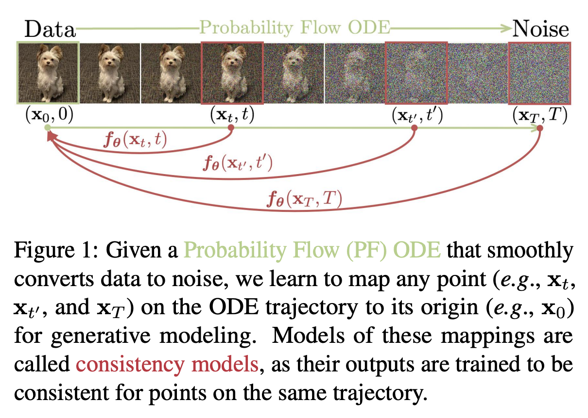
As mentioned at the beginning of this article, consistency models can achieve the mapping of any \(x_t \rightarrow x_0\), the essence of which is to force \(f(x_t) = f(x_{t-1}) = x_0\), thus making single-step iteration of the diffusion model possible. As shown in the figure below, PF ODE can transform the noise distribution \(x_T\) into the image distribution \(x_0\), represented by the green line. Due to errors, models that have not been trained with consistency distillation cannot achieve the trajectory of \(x_t \rightarrow x_0\), and the distribution obtained in a single step will significantly deviate from the distribution obtained in multiple steps. However, consistency models can make the trajectory of \(x_t \rightarrow x_0\) as shown by the red curve in the figure. Next, we will introduce in detail the method by which consistency models distill the trajectory of the red curve.
Parameters Definition
We first define the relevant parameters for the consistency model. Given the trajectory of PF ODE \( \{x_t\}_{t\in[0,T]} \), we define the consistency function as \( f:(x_t,t)\rightarrow x_0 \). The consistency function has the property of self-consistency, meaning that the output for any pair \( (x_t,t) \) belonging to the PF ODE trajectory is consistent, for example, \( f(x_t,t)=f(x_{t'},t') \), where \( t,t'\in[0,T] \). As shown in the figure below, the goal of the consistency model \( f_\theta \) is to force the model to learn the self-consistent property, estimating the ideal consistency function \( f \) from data.

We define the consistency function to satisfy \( f(x_0,0)=x_0 \). For the consistency model \( f_\theta \) based on deep neural networks, we use skip connections to parameterize the consistency model, that is:
$$ f_\theta(x,t)=c_{\text{skip}}(t)x+c_{\text{out}}(t)F_\theta(x,t), $$where \( c_{\text{skip}}(t) \) and \( c_{\text{out}}(t) \) are differentiable functions, for example, \( c_{\text{skip}}(0)=1, c_{\text{out}}=0 \). In this way, if \( F_\theta(x,t), c_{\text{skip}}(t), c_{\text{out}}(t) \) are differentiable, the consistency model is differentiable at \( t=0 \) .
Sampling Process
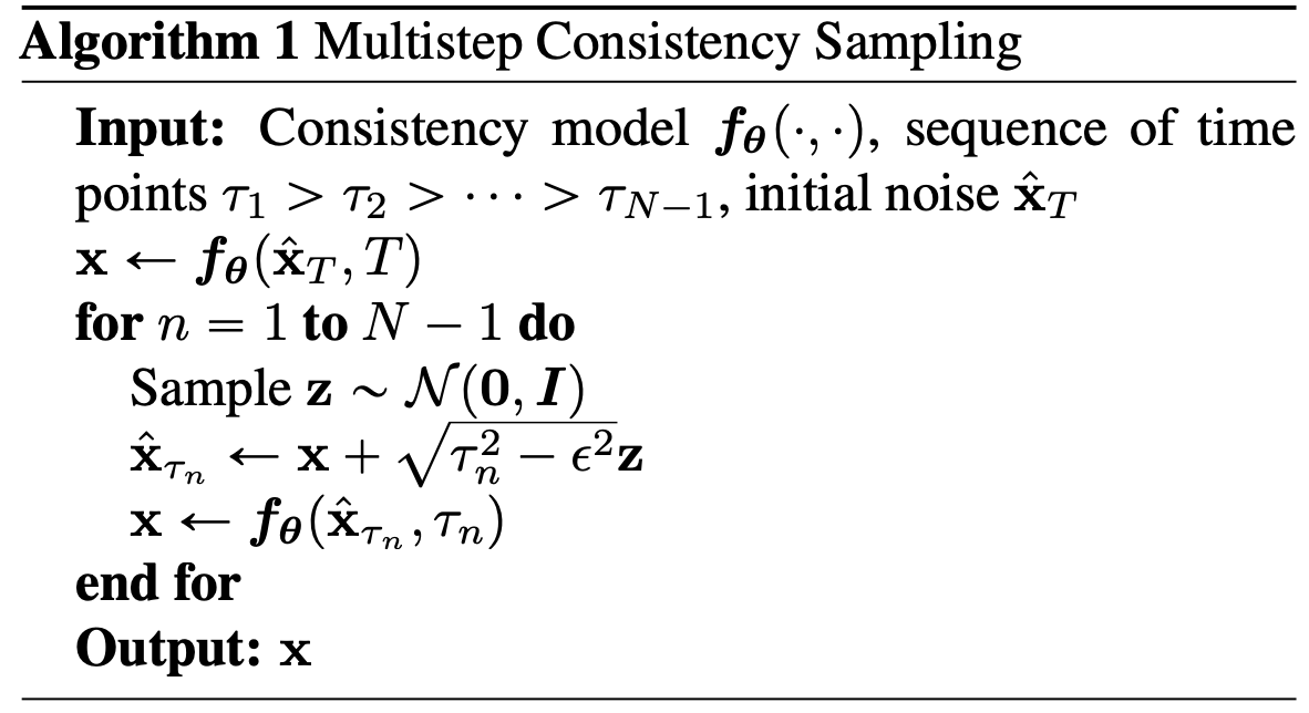
With a well-trained consistency model \( f_\theta(\cdot,\cdot) \), we can sample images from the initial distribution \( x_T\sim \mathcal{N}(0,T^2I) \). This sampling process involves only one forward pass of the consistency model, thus generating images in one step. More importantly, the consistency model can perform multiple alternating denoising and noise addition steps to improve image quality. The specific details are shown in the figure below, where the multi-step sampling process provides flexibility in balancing computation and sampling quality. However, in practice, the number of sampling steps for the consistency model does not exceed 8 steps. This is because the stochastic Gaussian noise in the noise addition process has uncertainty.
Training Process
The consistency model offers two training schemes: distillation and non-distillation, with the performance of distillation far exceeding that of non-distillation. Therefore, we focus on introducing the distillation training scheme.
For the distillation scheme, we propose training the consistency model based on a pre-trained score model \( s_\phi(x,t) \). Considering discretizing the continuous time \( [0,T] \) into \( N-1 \) sub-intervals, with boundary conditions satisfying \( t_1=0 More specifically, given a piece of data \( x \), we can use an ODE solver on the PF ODE trajectory to generate a neighboring data pair \( (x_{t_n}^\phi, x_{t_{n+1}}) \) in one step from \( x_{t_{n+1}} \) . After that, we train the consistency model by minimizing the distance between the consistency model output and \( (x_{tn}^\phi, x_{t_{n+1}}) \) . This prompts us to propose a consistency distillation loss for training the consistency model, that is: In the consistency model, \( d(\cdot) \) can be an \( \mathcal{l}_2, \mathcal{l}_1 \) loss, or LPIPS loss, and \( \lambda(t_n)=1 \) at any timestep. Our consistency model parameters are \( \theta \) , updated with EMA to stabilize the training process as \( \theta^- \) . That is, given a decay rate \( 0<\mu<1 \) , we perform the following update at each optimization step: Here, we provide a theoretical asymptotic analysis of consistency. If the consistency function \( f_\theta \) satisfies the Lipschitz condition, then there exists \( t \in [0,T], x, y \) such that \( ||f_\theta(x,t) - f_\theta(y,t)|| < L ||x - y||_2 \). Assuming \( n \in [1, N-1] \), the ODE solver has a local error at \( t_{n+1} \) of \( O((t_{n+1} - t_n)^{p+1}) \). If \( \mathcal{L}_{CD}^N(\theta, \theta; \phi) = 0 \), we have: In layman’s terms: We first define hypothetical conditions, then assume that the consistency function \( f_\theta(x, t) \) satisfies the Lipschitz condition, then consider that the ODE solver has a local error at \( t_{n+1} \), and is limited by \( O((t_{n+1} - t_n)^{p+1}) \). When the consistency distillation loss function \( \mathcal{L}_{CD}^N(\theta, \theta; \phi) = 0 \), we can achieve that the model’s output at each timestep \( f_\theta(x, t_n) \) approximates the theoretical output \( f(x, t_n; \phi) \) infinitely. Since when the training model converges, we have \( \theta^- = \theta \). Therefore, by minimizing the consistency distillation loss function, we can obtain a consistency model that approximates the theory. What is the Lipschitz condition? The Lipschitz condition assumes that the consistency model \( f_\theta \) satisfies the Lipschitz condition, meaning there exists a non-negative real number \( L \) such that for all timesteps \( t \) and any two points \( x, y \), the rate of change of the function \( f_\theta \) is bounded. What is asymptotic analysis? If the consistency distillation loss is 0, as the timestep difference \( \Delta t \) tends to zero and \( N \rightarrow \infty \), the model’s output at each timestep \( f_\theta(x, t_n) \) approximates the theoretical output \( f(x, t_n; \phi) \) infinitely. For more specific details, readers can refer to the appendix of the original text. [1] Song, Y., Dhariwal, P., Chen, M., & Sutskever, I. (2023). Consistency models. arXiv preprint arXiv:2303.01469.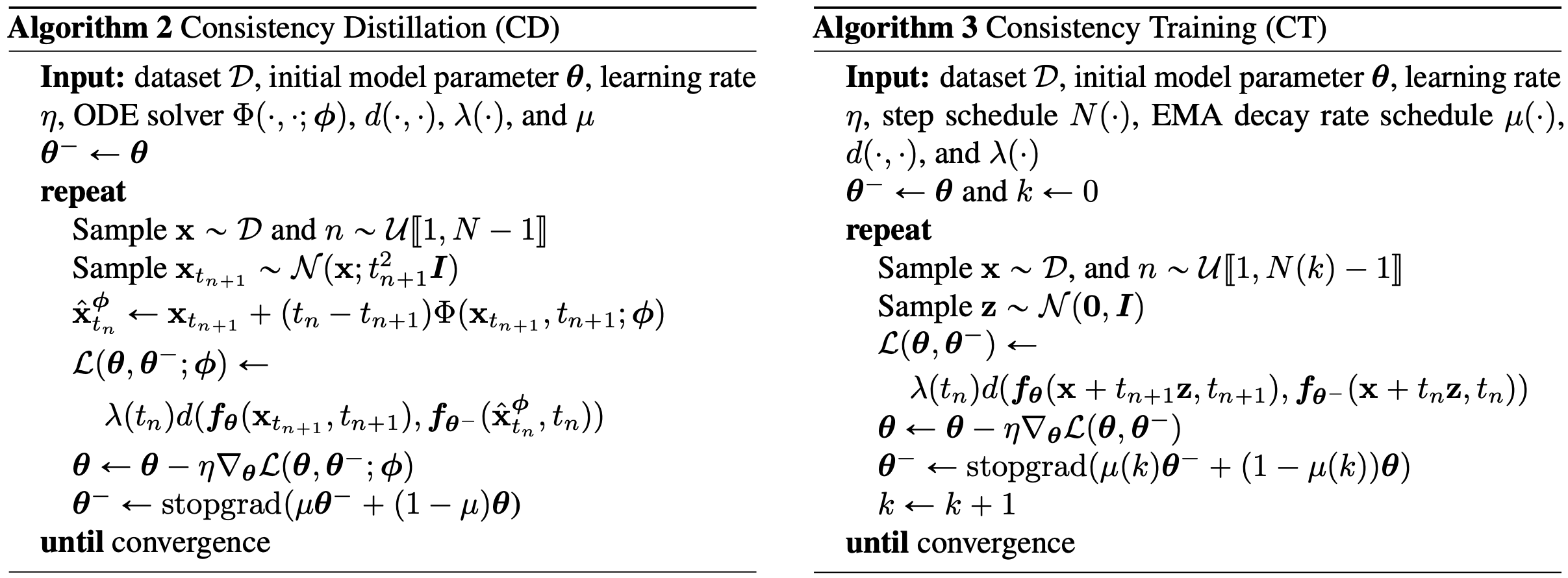
Asymptotic Analysis of Consistency Distillation
Reference